Simple Analytical min-max Model Matching Approach to Robust PID Tuning

A simple negative feedback control loop makes the process variable close to the set-point even if there are disturbances. The common strategy is to develop a mathematical model of the process and, based on it, to select appropriate values for the control algorithm parameters. In contrast with many empirical methods, this communication proposes the analytical tuning of a commercial PID controller based on a FOPDT model. The objective is to obtain smooth responses.
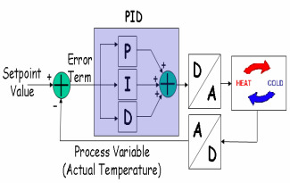
A simple negative feedback control loop has two major components: the process P and the controller K. The process has one input, the manipulated variable, also called the control variable and denoted by u. The process output is called process variable and is denoted by y.
This variable is measured by a sensor. The purpose of the system is to keep the process variable close to the desired value. The desired value of the process variable is called the set-point or the reference value and it is commonly denoted by r. Consequently, the objective of the control system amounts to keep the error signal e = r - y small (ideally zero) in spite of disturbances, denoted by d. The controller K has one input, the error e, and one output, the control variable u.The idea of feedback, yet simple, is extremely powerful. A simple and practical example is a thermostat: when the temperature in a heated room reaches a certain upper limit ( r + e ) the room heating is switched off so that the temperature begins to fall. When the temperature drops to a lower limit ( r - e ), the heating is switched on again. This way, a steady room temperature (r) can be maintained. This simple feedback mechanism can be described mathematically as follows:
where umax denotes the (constant) control action used when the heating is on. This type of feedback is called on-off control and it illustrates well the basic principle of negative feedback, present in many biological processes (think about the way our body temperature is maintained). The reason why feedback systems are of interest is that feedback makes the process variable close to the set-point even if there are disturbances (this is what happens when someone opens a window in the room of our thermostat example, making the temperature to change suddenly) and variation of the process characteristics (in our example, this represents the way in which the temperature changes in the room when the heating acts). Although the on-off control may be useful in some situations, the most standard industrial algorithm can be expressed as follows:
This controller combines three basic actions on the error signal: proportional, integrative and derivate and hence its name: Proportional-Integrative-Derivative (PID) controller. There is a problem with the ideal controller above: the derivative cannot be implemented in practice. Due to this fact, the standard, commercial algorithm is slightly different and a new parameter: , appears. Its role is that of making the system less sensitive to measurement noise. The procedure of finding the PID parameters (K, Ti, Td, N) is called tuning. Despite the fact that there already exist many PID tuning rules, new ones continue to appear year after year. This can be explained by the widespread use of PID control. The common strategy is to develop a mathematical model of the process and, based on it, to select appropriate values for the PID parameters. It is convenient to choose the simplest possible. In this vein, a very simple and representative three-parameter model for the process P is the First Order Plus Dead Time (FOPDT) one. Its response to a unit step signal, defined as
is depicted in the next figure
where Kp, t, h denote, respectively, the gain, time constant, and the dead-time (or delay) of the process. The time constant is the time it takes for the output of the system to reach the 63.2% of its steady-state value (Kp) once the dead-time (h) has elapsed. In the figure, Kp= t = h = 1. If we assume that the temperature distribution is quite homogenous in the room of our thermostat example, the above figure could taken as a lumped-parameter model for the variation of the temperature when the heater increases the heat transfer in a step fashion.
In contrast with many empirical methods, this communication proposes the analytical tuning of a commercial PID controller based on a FOPDT model. The objective is to obtain smooth responses: we want the control system to follow the reference as fast as possible while avoiding overshoot (this means that the output y is never greater than the specified reference r) and yielding good robustness. We say that a control system is robust if it continues to perform well when the real process differs (to a certain extent) from the process model, which is always the case in practice. The smoothness of the desired responses automatically prevents the manipulated variable to move too rapidly, reducing tear and wear on equipment.
References
"Simple Analytical min-max Model Matching Approach to Robust Proportional-Integrative-Derivative Tuning with Smooth Set-Point Response". Alcántara, S; Pedret, C; Vilanova, R; Zhang, WD. INDUSTRIAL & ENGINEERING CHEMISTRY RESEARCH, 49 (2): 690-700 JAN 20 2010.

